PINNs Part 2: Solving the Infinite Square Well Schrodinger Equation
06/28/2025
What interests me most about the physics informed neural network (PINN) is its potential to approximately solve differential equations representing a wide range of different physical phenomena. I decided to see if the methods described in PINNs Part 1: Existing Work could be extended to solve the Schrodinger equation (note that it's actually Schrödinger, but I don't have a "ö" on my keyboard, so I'm typing Schrodinger for the rest of this writeup). The original PINNs paper claims that their approach can be used to solve general non-linear partial differential equations. The Schrodinger equation, on the other hand, is a linear eigenvalue problem, and presents new challenges to the PINN approach. I undertook and ultimately overcame most of these challenges over the course of a few months.
All code used for this writeup can be found in this GitHub repo.
Particles and the Schrodinger equation
At a fundemental level, everything we humans physically interact with is some conglomeration of atoms (humans are a conglomeration of atoms too, of course). Atoms make up stuff. All stuff that is stuff, is composed of atoms which interact with each other in interesting and unintuitive ways. Every atom has a nucleus that contains neutron(s) and proton(s) that is surrounded by a "cloud" of electron(s). The electron is a fundamental particle of nature and understanding its physical behavior requires one to solve the Schrodinger equation.
In the world of quantum mechanics, reality is strange and probabilistic. When talking about a particle that follows the laws of quantum mechanics, you can't say where the particle is and what it is doing, but where it probably is and what it probably is doing. All information and derivations in this section come from Introduction to Quantum Mechanics (Third Edition) by David J. Griffiths and Darrell F. Schroeter, a surpirsingly readable textbook.
A particle is defined by its wavefunction, $\Psi$. The wavefunction is defined by the time-dependent Schrodinger equation
$$\begin{eqnarray}i \hbar \frac{\partial}{\partial t} \Psi = \hat{H}\Psi ,\end{eqnarray}$$
where $i$ is the imaginary number, $\hbar$ is the reduced Planck's constant, and $\hat{H}$ is the Hamiltonian operator. Solving this equation for $\Psi$ gives the state of the particle which can be operated on to determine the probability of its position and momentum. Where this equation comes from is beyond the scope of this writeup, but if you're so inclined, you can read Schrodinger's original proposal of the equation here (though, you may need to have read a quantum mechanics textbook to get what he's talking about, and even then, it's still not simple).
For more reasons I won't explain, a separation of variables allows the Schrodinger equation to be split into different position and time-dependent terms. I'll skip some more details and tell you that the time-independent (and position-dependent) Schrodinger equation is
$$\begin{eqnarray} \hat{H}\psi = E\psi , \end{eqnarray}$$
where $\psi$ is the time-independent wave function and $E$ is the energy eigenvalue. This writeup only focuses on the time-independent Schrodinger equation.
This PDE can be solved by finding an eigenfunction $\psi$ and its corresponding eigenvalue $E$. Notice that we will look for a solution, not the solution. That is because this is a linear PDE. When a PDE is linear, it basically means that if you find a solution, you can multiply that solution by some constant and get another solution, meaning there are infinitely many solutions (since there are infinitely many constants).
There are two unknowns to find when solving the Schrodinger equation: the eigenfunction, $\psi$, and the corresponding energy eigenvalue, $E$. This differs from the original PINNs paper because it only focuses on predicting the function that solves a differential equation.
The remainder of this writeup focuses on adapting the PINNs technique to solve the Schrodinger equation applied to a common system presented in quantum mechanics textbooks in 1D, 2D, and 3D.
Adapting the PINN approach to a linear eigenvalue problem
Similar to the approach taken to solve Burger's equation in Part 1, the goal here is to train a neural network to predict a $\psi$ that satisfies the Schrodinger equation using position as an input.
But there's a problem: we have another unknown to find, $E$.
I searched for other papers that use PINNs to solve eigenvalue problems and found Physics-Informed Neural Networks for Quantum Eigenvalue Problems by Jin, Mattheakis, and Protopapas to be the most relevant. I also found an older/slightly different version here which explains certain parts of the other paper a bit more in-depth.
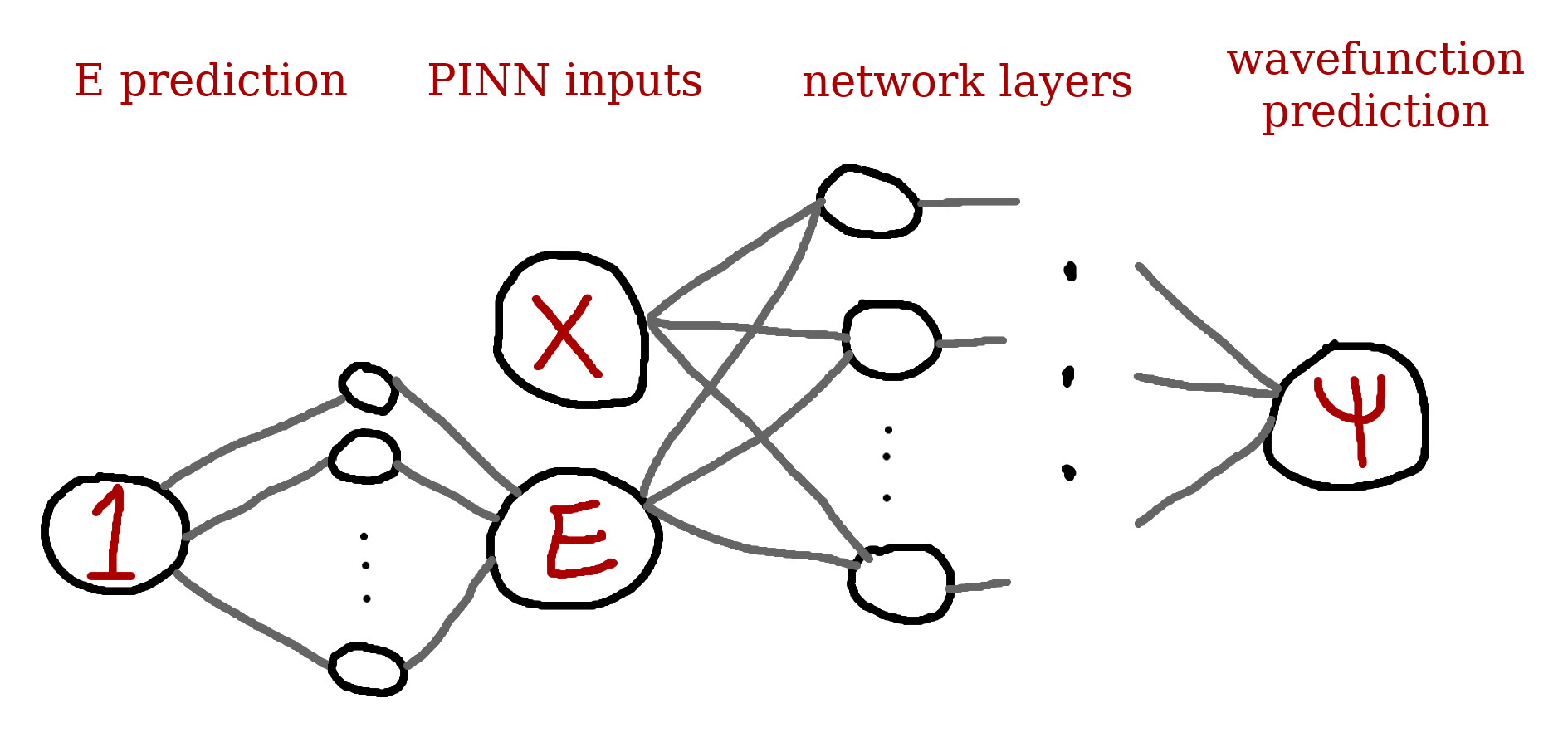
This paper proposes using an affine layer (dense layer that takes 1 as an input and produces a single output) at the start of the network to predict $E$, and then combines $E$ with position data ($x$ in this 1D example) as the input to the PINN. This creates a trainable layer in the PINN for finding $E$.
To find the energy eigenvalue along with the wavefunction, the authors introduce the loss term,
$$\begin{equation} L_{drive} = e^{-E + c}, \end{equation}$$
to promote the discovery of a correct $E$. The term $c$ is a value that is incremented across training to promote larger values of $E$. In practice, the PINN's predictions are penalized heavily when $E \lt c$ and $L_{drive}$ is "more satisfied" when $E \ge c$. Since there are infinitely many solutions to the differential equation, we have to scan across values of $E$ to find $\psi$ solutions. The aforementioned paper scans across $E$ values by incrementing $c$ across training. I implemented this method in my own code and was able to replicate their success. However, I found that $L_{drive}$ depended heavily on the amount that $c$ was incremented by across training and the initial value of $E$. Effectively, this loss term makes the network scan across values of $E$ in whatever increment of $c$ you decide across training. I realized that this is just a more complicated way to search across a bunch of pre-determined $E$ values with the added detriment that $L_{drive}$ has a tendency to blow up if the network does not adjust its predicted value of $E$ quickly enough. This "explosion" in $L_{drive}$ often appeared to have led to inconsistent results in training, though the network did learn to adjust its $E$ prediction correctly most of the time.
So, I decided to ditch the approach with $L_{drive}$ and simply scan across a range of $E$ values during training instead. The basic algorithm:
- set minimum value of $E$, $E_{min}$, and maximum value of $E$, $E_{max}$
- generate set of $E$ values ranging from $E_{min}$ to $E_{max}$ in step size $\delta_E$
- iterate across set of $E$ values, fully train PINN with each $E$ as a fixed input, calculate and save loss values
- after training PINNs on all values of $E$, determine which PINN(s) + value(s) of $E$ satisfy loss constraints the best
is simple, and maybe a bit computationally inefficient, but proves effective. This algorithm requires you to roughly know the expected range of energy values your system can have along with an appropriate energy increment, $\delta_E$.
All PINNs used in the problems below are simple, fully-connected feed-forward neural networks that make use of a sin activation function.
1D Infinite Square Well
Imagine that a particle is confined to exist in the 1D space $x \in [0, a]$. The particle cannot escape this space because it does not have enough energy to overcome the boundaries of the "potential well" it is trapped in.
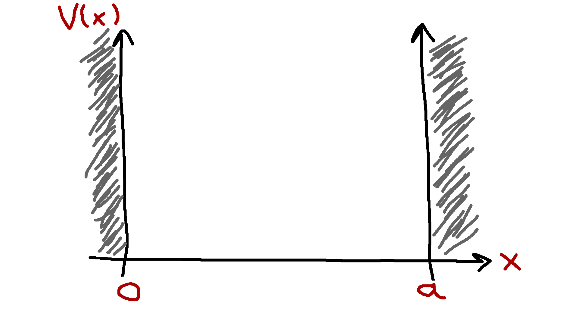
Formally, this system is described by the potential,
$$\begin{equation} V(x) = \begin{cases} 0, &0 \leq x \leq a \\ \infty, &\text{else} \end{cases}\end{equation}$$
and outside of the well,
$$\begin{equation} \psi(x) = 0. \end{equation}$$
The Hamiltonian operator, $\hat{H}$, is given,
$$\begin{equation} \hat{H} = -\frac{\hbar^2}{2m} \frac{d^2}{dx^2} + V(x),\end{equation}$$
where $m$ is the mass of the particle.
We know that the wavefunction of the particle is zero outside of the well, so we only concern ourselves with solving the equation when $V(x)=0$. After applying $\hat{H}$, we can write the Schrodinger equation,
$$\begin{equation} -\frac{\hbar^2}{2m} \frac{d^2 \psi}{dx^2} = E \psi.\end{equation}$$
The analytical solution is given,
$$\begin{eqnarray} \psi_n(x) &=& \sqrt{\frac{2}{a}} sin(\frac{n \pi}{a} x), \\ E_n &=& \frac{n^2 \pi^2 \hbar^2}{2 m a^2}, \end{eqnarray}$$
where $n \in [1, 2, ...]$ is the quantum number representing the energy level.
Okay, let's apply the new eigenvalue PINN algorithm to this problem.
First, we need to define to define the units of $x$, $\hbar$, and $m$. To keep things simple, I will use Coulomb units, which define the physical dimensions,
$$\begin{eqnarray} \text{mass} &=& m \text{ (electron)}, \\ \text{length} &=& \frac{\hbar^2}{mC}, \\ \text{energy} &=& \frac{mC^2}{\hbar^2}, \end{eqnarray}$$
which allows us to set,
$$\begin{equation} m=\hbar=C=\frac{e^2}{4 \pi \varepsilon_0}=1 .\end{equation}$$
This lets us write,
$$\begin{equation} \frac{\hbar^2}{2m} = \frac{1}{2},\end{equation}$$
and the energy level can be expressed as
$$\begin{equation} E_n = \frac{n^2 \pi^2}{2a^2} . \end{equation}$$
We can just arbitrarily call our units of $x$ to be length from $0$ to $a$.
These units are nice because they give the constants an appropriate order of magnitude (I invite you to check out these constants in SI units), but it took me an incredibly long time to figure out the correct unit system and I experienced an endless amount of issues as a consequence. For the infinite well problem, defining all of these units correctly isn't a big deal because there is only one constant term in the differential equation, but these definitions become very important for differential equations that contain multiple fundamental constants.
Next, we need to generate input data. This is easy, let $a=1$ and simply generate values of $x$ between $0$ and $a$. In practice, I generated $x$ values in steps of $0.01$. During training, all $x$ are perturbed by a small amount of noise and then passed into the PINN. The perturbation of inputs prevents the model from overfitting.
Note that we haven't generated a set of collocation and boundary condition data like in the original PINNs paper. I opted to just use collocation data and scale the PINN predictions to $0$ at the boundaries using the parametric scaling function presented in the quantum eigenvalue paper,
$$\begin{equation} g(x) = (1 - e^{-(x - x_{min})}) (1 - e^{x - x_{max}}) \end{equation},$$
where $x_{min}=0$ and $x_{max}=a$. Given a PINN output $u(x)$, the final prediction of the wavefunction, $\hat{\psi}(x)$, is given by,
$$\begin{equation} \hat{\psi}(x) = g(x)u(x). \end{equation}$$
Letting $\hat{\psi}$ represent the PINN's predicted wavefunction value and moving all terms of the differential equation to one side,
$$\begin{equation} f = E \hat{\psi} + \frac{\hbar^2}{2m} \frac{d^2 \hat{\psi}}{dx^2} .\end{equation}$$
The gradients are again calculated using PyTorch's autograd functionality. The differential equation loss is defined,
$$\begin{equation} L_{f} = \frac{1}{n_{f}} \sum_{i=0}^{n_{f}} f_i^2 , \end{equation}$$
where $n_f$ is the number of predictions and $f_i$ is the $f$ calculation of the $i$th prediction.
In addition to this loss term, I define a regularization term that penalizes trivial predictions,
$$\begin{equation} L_{trivial} = \frac{1}{\frac{1}{n_f} \sum_{i=0}^{n_f} {\hat{\psi_i}}^2} . \end{equation}$$
The overall loss of the network's predictions is,
$$\begin{equation} L = L_{f} + L_{trivial} . \end{equation}$$
$L$ cannot reach $0$ because of $L_{trivial}$. $L_{f}$ is the actual measure of the PINN's performance, but $L_{trivial}$ is necessary to keep the PINN from predicting $0$ for every input (the easiest way to minimize $L_{f}$).
For physics reasons that I won't get into, wavefunctions must be orthonormal to each other,
$$\begin{equation} \int \psi_{m}(x) * \psi_{n}(x) dx = \delta_{mn} . \end{equation}$$
For a single solution in the 1D well, $\psi$, this means,
$$\begin{equation} \int_{0}^{a} |\psi(x)|^2 dx = 1 . \end{equation}$$
I tried to introduce a loss term that incentivizes the PINN to predict normalized wavefunctions, but couldn't seem to get good prediction convergence. I also experimented with a transfer learning technique that was able to produce a normalized prediction, but that approach felt like a bit of a work-around/hack, so I dropped it.
With the aforementioned loss terms, the PINN was able to predict correct values of $E$ alongside the correct shapes of the corresponding wavefunctions. But, these wavefunctions did not meet the normalization condition and appeared to be scaled versions of the normalized analytical solutions. I had a hunch that,
$$\begin{equation} \psi = c \hat{\psi},\end{equation}$$
where $\psi$ is the true analytical soluion, $\hat{\psi}$ is the PINN's prediction, and $c$ is some unknown constant that relates the two wavefunctions. I will call $c$ the "prediction normalization constant."
With this assumption and the normalization condition, I figured that I could find the approximate value of $c$, and thus derive an approximate analytical solution from the prediction without knowing the analytical solution itself.
The normalization condition integral can be approximated with a sum across all $x$ values in our system's domain,
$$\begin{equation} \sum_{i=0}^{n_a} \psi^2(x_i)\delta_x \approx 1, \end{equation}$$
where $n_a$ is the number of $x$ values in the approximate domain, $x_i$ is the $i$th $x$ value in the approximate domain, and $\delta_{x}$ is the step size between each $x_i$.
From the assumed relationship between $\psi$ and $\hat{\psi}$,
$$\begin{eqnarray} \sum_{i=0}^{n_a} \psi^2(x_i)\delta_x &\approx& c^2\sum_{i=0}^{n_a}\hat{\psi}^2(x_i)\delta_x \\ \Rightarrow c &\approx& \frac{1}{\sqrt{\delta_x \sum_{i=0}^{n_a} \hat{\psi}^2(x_i) }} \end{eqnarray}$$
This equation looks more complicated than it actually is. All this equation says is, "for each $x_i$ in the set $[x_0, x_1, ..., x_{n_a}]$, get the prediction $\hat{\psi}(x_i)$, square it, sum all of those squared predictions up, then take 1 divided by the square root of that sum to get $c$."
This may seem like a convoluted way to get a normalized prediction, but it works if the assumption $\psi = c \hat{\psi}$ holds, and I feel like it's clever, so, this is what I stuck with.
With all of the above defined, the PINN can finally be trained. I scanned across $E$ values from $1$ to $23$ in $\delta_E$ increments of $0.1$, training a PINN on each value of $E$ with $1000$ training steps. The following video illustrates how the PINN learned solutions across training (note that $\hat{u} \equiv \hat{\psi}$ and Schrodinger loss $\equiv L_{f}$ in the plots).
The training progress video above scans across the first three known analytical solution $E$ values. You can see how the $L_{f}$ of the PINN's predictions drops steeply when the PINN is trained on the correct analytical $E$ values.
I don't love the algorithm I came up with to search over $E$ values because it is computationally inefficient. In the training above, I fit 230 PINNs (230 $E$ values scanned), and find 3 approximately correct solutions. I'd like to say I had some revelation that led me to develop a better method to determine $E$, but that didn't happen.
The training above increments $E$ by a fairly large step, $0.1$, and may not allow the network to find accurate-enough solutions since I can't guarantee a correct value of $E$ beyond a single decimal place. This made me wonder if I could run a wide search over $E$ like above, and then "zoom in" on the values of $E$ that the PINN made the best wavefunction predictions with.
The PINNs trained above converged on $E_1=2.4$, $E_2=9.4$, and $E_3=21.1$. The corresponding correct analytical solutions to two decimal places are $E_1=2.35$, $E_2=9.39$, and $E_3=21.12$, respectively. I retrained on $E$ values between $[2.3, 2.5]$, $[9.3, 9.5]$, $[21, 21.2]$ in $E$ increments of $0.01$. As expected the PINNs were able to find the correct wavefunctions with greater accuracy in $E$. The PINNs converged to best predictions on $E_1=2.35$, $E_2=9.40$, and $E_3=21.12$. This process of retraining and "zooming in" on the best found $E$ values can be extended to attain even higher levels of accuracy in determining $E$.
To visualize the PINN's convergence to the analytical solutions more clearly, here is a video showing training that only searches over the first three analytical $E$ values very closely alongside the nearest correct analytical solution.
In the video above, I plot the non-normalized prediction, analytical solution (normalized by definition), and sign-corrected normalized prediction. The PINN sometimes predicts the negative version of the correct wavefunction, which still solves the Schrodinger equation the same as the positive version, it's just a convention to use the positive version when writing the analytical solution. I flip signs where relevant above for a better visualization. You can see how the dashed green line almost perfectly overlaps with the analytical solution, qualitatively indicating solid PINN convergence. Quantitatively, the three best PINNs trained above attain $L_{f}$ values on the order of $10^{-3}$ to $10^{-2}$. This is comparable to the results attained in the original PINNs paper as described in Part 1.
Since I have the analytical solution for this problem, the MSE on predictions is easy to calculate. The MSE values for each PINN's predictions above are on the order of $10^{-4}$, $10^{-3}$, and $10^{-2}$, respectively. It seems like the PINN's accuracy decreases with increasing $n$, but this might just be an indicator that the PINN needed more time to converge to a correct solution.
All code used for this section can be found in this notebook.
2D Infinite Well
To extend the infinite well problem to 2D, we say that the particle is now trapped in a rectangle in the xy plane. For simplicity's sake, we'll say this rectangle is a square of dimensions $a$ x $a$.
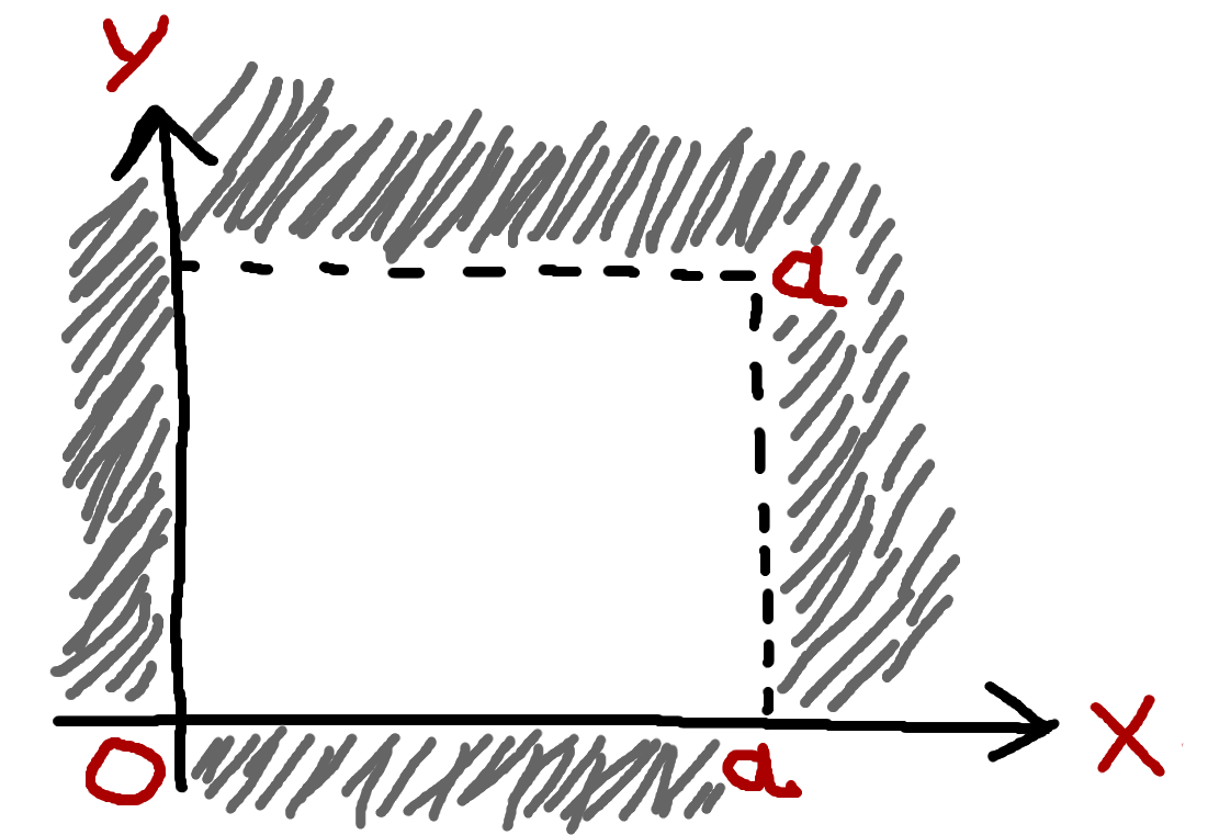
Formally,
$$\begin{equation} V(x, y) = \begin{cases} 0, &0 \leq x \leq a \text{ and } 0 \leq y \leq a \\ \infty, &\text{else} \end{cases}\end{equation}$$
and outside of the well,
$$\begin{equation} \psi(x, y) = 0. \end{equation}$$
The Hamiltonian operator is now,
$$\begin{equation} \hat{H} = -\frac{\hbar^2}{2m} (\frac{\partial^2}{\partial x^2} + \frac{\partial^2}{\partial y^2}) + V(x, y).\end{equation}$$
Once again, we only care about the region where the particle's wavefunction is non-zero and $V(x, y) = 0$, so the Schrodinger equation becomes,
$$\begin{equation} -\frac{\hbar^2}{2m} (\frac{\partial^2 \psi}{\partial x^2} + \frac{\partial^2 \psi}{\partial y^2}) = E \psi.\end{equation}$$
The analytical solution is given,
$$\begin{eqnarray} \psi(x, y) &=& \frac{2}{a} sin(\frac{n_x \pi}{a}x) sin(\frac{n_y \pi}{a}y), \\ E_n &=& \frac{\hbar^2 \pi^2}{2ma^2} (n_x^2 + n_y^2), \end{eqnarray}$$
for quantum numbers $n_x \in [1, 2, ...]$ and $n_y \in [1, 2, ...]$. I'll define $n=n_x^2 + n_y^2$ and $N=n_x + n_y$ to keep track of the specific energy level.
It is interesting to note that the additional dimension in this problem results in degenerate states in each energy level. This means there can be multiple valid wavefunctions that solve the Schrodinger equation with the same energy eigenvalue. For simplicity's sake, I aim to train a PINN to find a single solution for each energy level, and just accept that degenerate states exist and that the PINN can converge to different correct wavefunctions for the same $E$.
Initially, I tried to handle the boundary conditions of this problem with an altered version of the parametric scaling function described in the 1D section. I couldn't seem to get the PINN to converge to good results with this method, so I went back to using the method of defining collocation and boundary condition data that the original PINNs paper introduced. I somewhat arbitrarily decided on a 10:1 split of collocation:boundary condition data points.
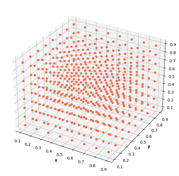
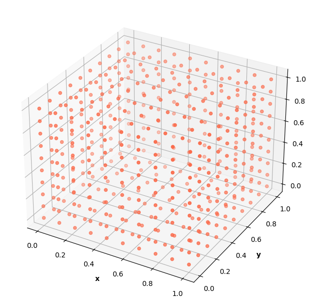
The boundary data outlines the well:
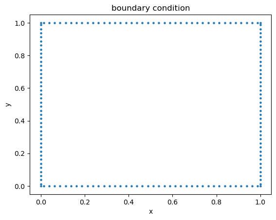
The collocation data contains points inside the well:
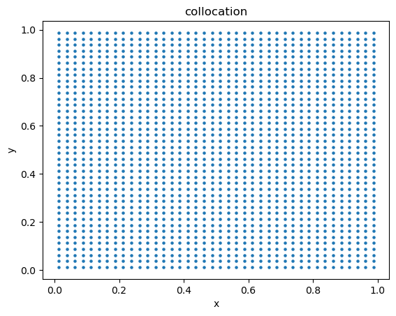
As the number of dimensions increases, the amount of data required to respresent the space of our system increases. Determining a reasonably small enough step size betwen each point in the square above is a matter of experimentation and introduces a tradeoff. On the one hand, you want to generate enough data to represent your system, but on the other hand, you don't want to generate too much data because that may require the PINN to train for an unreasonable amount of time in order to achieve good convergence.
Again, $f$ is defined by moving all terms in the Schrodinger equation to one side,
$$\begin{equation} f = E \hat{\psi}_f + \frac{\hbar^2}{2m} (\frac{\partial^2 \hat{\psi}_f}{\partial x^2} + \frac{\partial^2 \hat{\psi}_f}{\partial y^2}) ,\end{equation}$$
where $\hat{\psi}_f$ represents the PINN's predicted wavefunction value on a collocation point. The corresponding loss is defined,
$$\begin{equation} L_{f} = \frac{1}{n_{f}} \sum_{i=0}^{n_{f}} f_i^2 . \end{equation}$$
With the re-introduction of the b.c. + collocation data split, $n_f$ now represents the number of data points in the collocation data set and $n_{bc}$ represents the number of points in the b.c. data set. The loss for the b.c. data is the same MSE used from the original PINNs paper,
$$\begin{equation} L_{bc} = \frac{1}{n_{bc}} \sum_{i=0}^{n_{bc}} \hat{\psi}_{bc, i}^2 , \end{equation}$$
where $\hat{\psi}_{bc, i}$ is the PINN's prediction of the $i$th b.c. data point.
The trivial prediction loss term only applies to predictions made on points in the collocation data set (since the prediction at the b.c. is supposed to be 0),
$$\begin{equation} L_{trivial} = \frac{1}{\frac{1}{n_f} \sum_{i=0}^{n_f} {\hat{\psi}_{f, i}}^2} . \end{equation}$$
The overall loss is now defined,
$$\begin{equation} L = L_{f} + L_{bc} + L_{trivial} . \end{equation}$$
The normalization condition for this problem is,
$$\begin{equation} \int \int |\psi(x, y)|^2 dxdy = 1. \end{equation}$$
The same logic described in the 1D case above can be extended to update the prediction normalization constant calculation,
$$\begin{eqnarray} \sum_{j=0}^{n_a} \sum_{i=0}^{n_a} \psi^2(x_i, y_j) \delta_x \delta_y &\approx& c^2 \sum_{j=0}^{n_a} \sum_{i=0}^{n_a}\hat{\psi}^2(x_i, y_j) \delta_x \delta_y \\ \Rightarrow c &\approx& \frac{1}{\sqrt{\delta_x \delta_y \sum_{j=0}^{n_a} \sum_{i=0}^{n_a} \hat{\psi}^2(x_i, y_j) }} \end{eqnarray}$$
Since we have a square of data where $\delta_x = \delta_y$, the double sum in the denominator becomes a single sum across all generated data points in code.
Through some trial and error, I found that the PINN required about 5 minutes of training to converge to a good-enough solution for a single value of $E$. Running a sufficiently large scan over enough $E$ values to find a few solutions requires several uninterrupted hours of training time. This is the main issue with the $E$ scan algorithm: it's computationally intensive and inefficient since you must scan over many incorrect $E$ values before the PINN finds a correct solution. In order to shorten the training time, I cheated a bit and just scanned over 3 $E$ values near the first 4 true $E$ values.
Since $L_{trivial}$ is just a regularization term meant to push the PINN to predict non-trivial solutions, I define the actual performance of the PINN by the loss term,
$$\begin{equation} L_{ovr} = L_{f} + L_{bc}. \end{equation}$$
In code I referred to this as "loss_ovr_no_reg,"
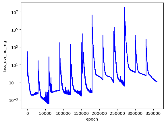
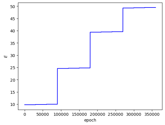
The analytical $E$ values for the first $4$ solutions are $9.87$, $24.67$, $39.48$, and $49.35$, respectively. In this training run, I set the scan to look over the values $E-0.1$, $E$, $E+0.1$ for each analytical $E$ (i.e. the first scan went across $9.77$, $9.87$, $9.97$). My hope was that the PINN would converge to the best $L_{ovr}$ on the middle $E$ value in each set of $3$ $E$ values.
Looking at the plot of $L_{ovr}$ above, you can see that the PINN does minimize $L_{ovr}$ with the correct $E$ for the first two energy levels, but fails to do so with the last two $E$ values. That being said, the PINN still finds very accurate wavefunctions for each energy level. The plots below show $\psi(x,y)$ in the z-axis and the color of each point is the probability density of the wavefunction, $|\psi(x,y)|^2$.

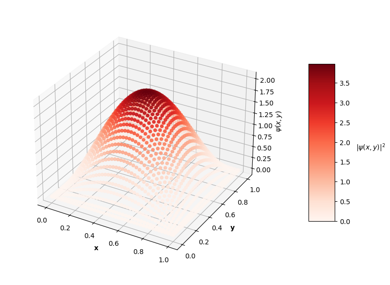

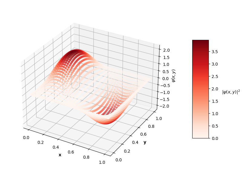

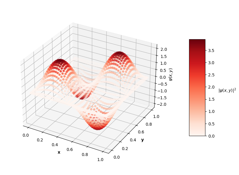
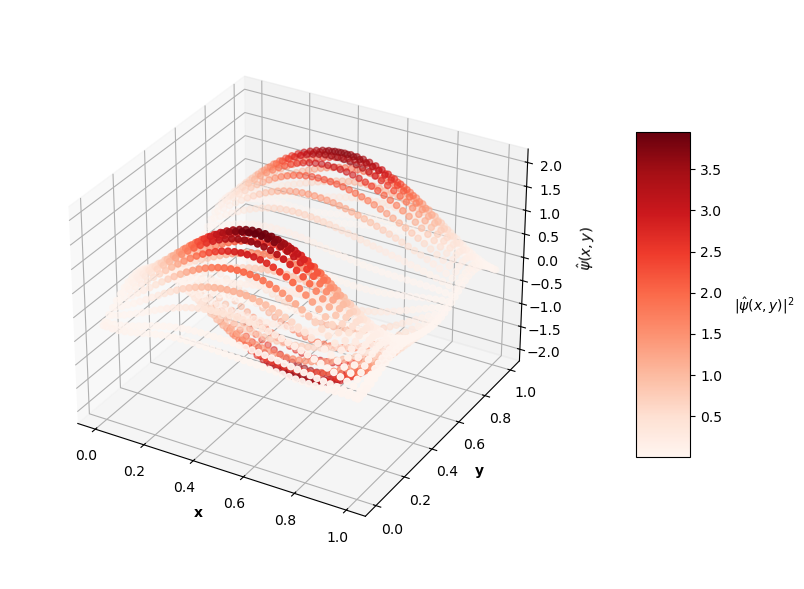
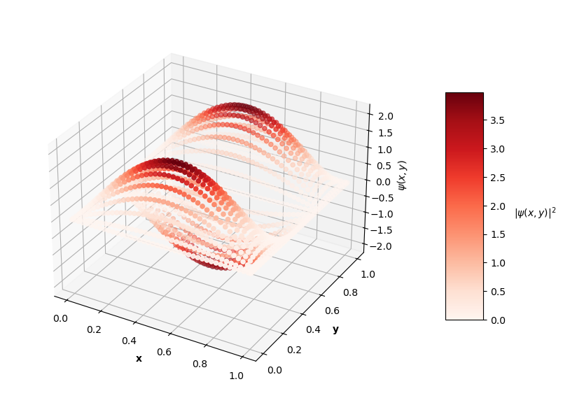
Visually, the predicted wavefunctions look identical to the analytical solutions. The Schrodinger equation loss ($L_{f}$) for these $4$ PINNs ranges between the orders of $10^{-4}$ to $10^{-2}$. The MSE values of these predictions against the analytical solutions range between the orders of $10^{-7}$ to $10^{-3}$.
It seems like the PINN has a harder time converging to good solutions with increasing $N$. Though, I could train these higher energy PINNs longer and could tune the hyperparameters of the network itself to achieve better results. Longer training time may result in the PINN finding the best solution with the correct $E$ value as well. For now, I'm satisfied with seeing some decent convergence here and am convinced that this PINN approach is effective enough, at least as a proof of concept.
All code used for this section can be found in this notebook.
3D Infinite Well
To extend the paricle in a well problem to 3D, we now say the particle is trapped in a 3D rectangular prism. For simplicity's sake, I use a cube of dimensions $a$ x $a$ x $a$ and let $a=1$. I'll leave the visualization to your own brain for this one.
Formally,
$$\begin{equation} V(x, y, z) = \begin{cases} 0, &0 \leq x \leq a, \text{ } 0 \leq y \leq a, \text{ } 0 \leq z \leq a \\ \infty , &\text{else} \end{cases}\end{equation}$$
and outside of the well,
$$\begin{equation} \psi(x, y, z) = 0. \end{equation}$$
Another gradient for the z dimension is added to the Hamiltonian,
$$\begin{equation} \hat{H} = -\frac{\hbar^2}{2m} (\frac{\partial^2}{\partial x^2} + \frac{\partial^2}{\partial y^2} + \frac{\partial^2}{\partial z^2}) + V(x, y, z).\end{equation}$$
We again only care about non-zero wavefunctions where $V(x, y, z)=0$, and the Schrodinger equation becomes,
$$\begin{equation} -\frac{\hbar^2}{2m} (\frac{\partial^2 \psi}{\partial x^2} + \frac{\partial^2 \psi}{\partial y^2} + \frac{\partial^2 \psi}{\partial z^2}) = E \psi.\end{equation}$$
The analytical solution is given,
$$\begin{eqnarray} \psi(x, y, z) &=& \sqrt{\frac{8}{a^3}} sin(\frac{n_x \pi}{a}x) sin(\frac{n_y \pi}{a}y) sin(\frac{n_z \pi}{a}z), \\ E_n &=& \frac{\hbar^2 \pi^2}{2ma^2} (n_x^2 + n_y^2 + n_z^2) .\end{eqnarray}$$
A cube of data points is generated to represent the 3D well that the particle exists in. Again, I generate sets of collocation and boundary condition data.
$f$ is defined,
$$\begin{equation} f = E \hat{\psi}_f + \frac{\hbar^2}{2m} (\frac{\partial^2 \hat{\psi}_f}{\partial x^2} + \frac{\partial^2 \hat{\psi}_f}{\partial y^2} + \frac{\partial^2 \hat{\psi}_f}{\partial z^2}) .\end{equation}$$
The prediction normalization constant calculation extends to a third dimension,
$$\begin{eqnarray} \sum_{k=0}^{n_a} \sum_{j=0}^{n_a} \sum_{i=0}^{n_a} \psi^2(x_i, y_j, z_k) \delta_x \delta_y \delta_z &\approx& c^2 \sum_{k=0}^{n_a} \sum_{j=0}^{n_a} \sum_{i=0}^{n_a}\hat{\psi}^2(x_i, y_j, z_k) \delta_x \delta_y \delta_z \\ \Rightarrow c &\approx& \frac{1}{\sqrt{\delta_x \delta_y \delta_z \sum_{k=0}^{n_a} \sum_{j=0}^{n_a} \sum_{i=0}^{n_a} \hat{\psi}^2(x_i, y_j, z_k) }} \end{eqnarray}$$
This looks like a mess, but again the triple summation in the denominator is reduced to a single sum across all data points in the cube in code because $\delta_x = \delta_y = \delta_z$.
The loss terms for this PINN are the same terms used in the 2D case.
Considering the large range of $E$ values in the first 4 analytical solutions to this problem, I once again only searched over $E$ values near the analytical $E$. The PINN was able to find correct-looking solutions for the first 3 energy levels, but did not converge to the correct $E$ value for each, and did not find the correct wavefunction for the 4th energy level.
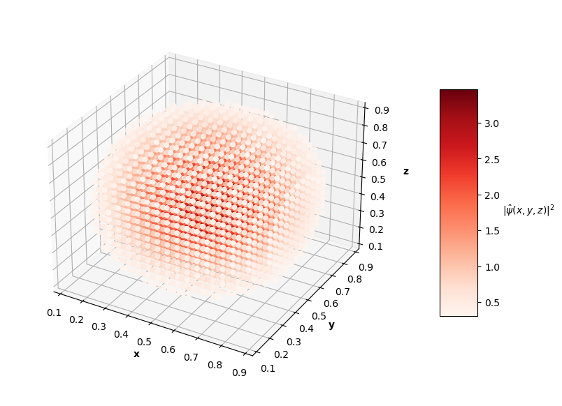
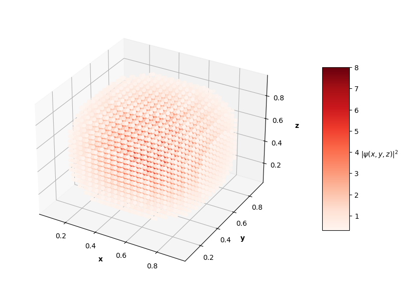
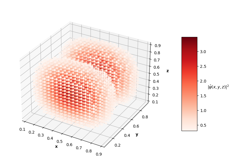
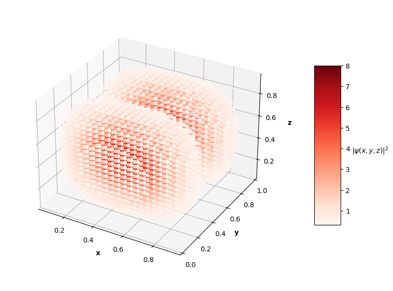
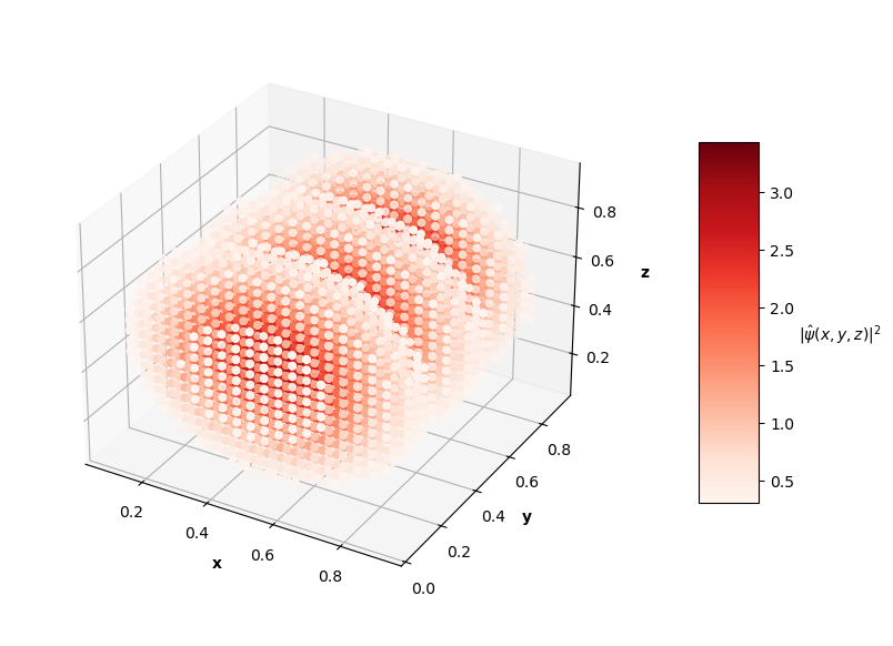
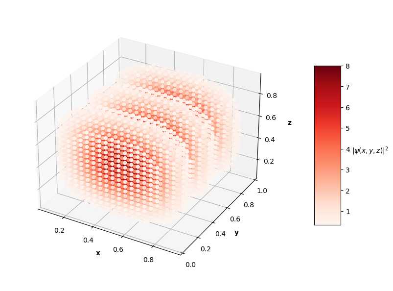
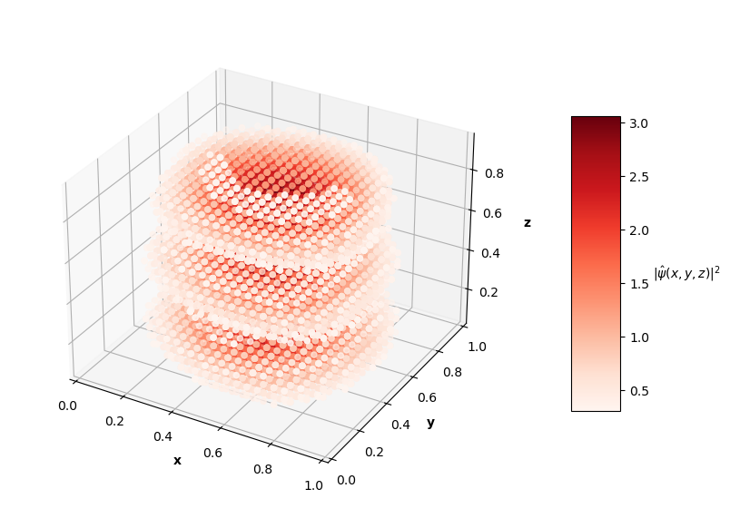
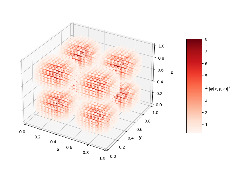
For visualization purposes, the plots above only show points that have probability densities above a certain threshold (you would just see an isometric view of a cube if I didn't subset the predictions and solutions).
The $L_f$ values on these predictions range from the order of $10^{-3}$ to $10^{-2}$ with analytical MSE values between $10^{-1}$ to $10^{0}$. In the prediction plots above, the predicted probability densities, $|\hat{\psi}(x, y, z)|^2$, appear to be half of the analytical solution's probability densities. I'm not sure if this is because of an error in my calculation of the prediction normalization constant or if the PINN just didn't learn the $\psi = c \hat{\psi}$ assumption like in the 1D and 2D problems. It's also interesting to note that the PINN in the $N=4$ case learned to predict the shape of a degenerate state of the $N=3$ solution (specifically the $n_x=1$, $n_y=1$, $n_z=3$ state). Clearly, this PINN approach struggled to converge to correct solutions as well as the 1D and 2D cases. Longer training time and more complex network architectures may help the PINN achieve better convergence as the dimensions of the input system increase.
All code used for this section can be found in this GitHub repo.
Limitations of this approach and next steps
As stated before, I don't love the $E$ search algorithm that I came up with and would much rather develop an approach that enables the PINN to learn both $E$ and $\psi$ on its own. The PINNs trained on the higher dimension infinite well problems struggled to make significantly better predictions when the correct $E$ value was used as an input, and $L_f$ was larger as the number of dimensions in the system increased.
In the 3D well problem described above, I decided not to focus on optimizing for best results and fixing the potential issues with the approach because I wanted to move onto implementing a PINN to solve the Hydrogen atom Schrodinger equation, a significantly more complicated 3D problem. For now, I'm satisfied with the proof of concept I've demonstrated here with this PINN approach and will further refine it in my future work.
If you want more, check out my next post on solving the Hydrogen atom Schrodinger equation with a PINN.