PINNs Part 3: Solving the Hydrogen Atom Schrodinger Equation
10/26/2025
To see if the PINN algorithm presented in Part 2 is capable of solving harder problems, I applied it to the Hydrogen atom Schrodinger equation. The Hydrogen atom consists of a nucleus and one electron. The Schrodinger equation is used to find the wavefunction of the electron.
The Hydrogen atom Schrodinger equation
The Hamiltonian operator for Hydrogen is defined
$$\begin{eqnarray} \hat{H} = -\frac{\hbar^2}{2m}\nabla^2 + V(\vec{r}) , \end{eqnarray}$$
where $\nabla^2$ is the Laplace operator, $m$ is the mass of the electron, and $V(\vec{r})$ is the potential of the electron defined by
$$\begin{eqnarray} V(\vec{r}) = -\frac{e^2}{4 \pi \varepsilon_0 |\vec{r}|} , \end{eqnarray}$$
where $\vec{r}$ is the position of the electron in 3D cartesian coordinates, $e$ is the charge of the electron, and $\varepsilon_0$ is the permittivity of free space.
Unlike the infinite square well differential equation, the Hydrogen atom Schrodinger has a non-zero potential term. This complicates the equation and makes it significantly harder to solve analytically.
The full Schrodinger equation is
$$\begin{eqnarray} -\frac{\hbar^2}{2m} \left(\frac{\partial^2 \psi}{\partial x^2} + \frac{\partial^2 \psi}{\partial y^2} + \frac{\partial^2 \psi}{\partial z^2} \right) - \frac{e^2}{4 \pi \varepsilon_0 |\vec{r}|}\psi = E\psi . \end{eqnarray}$$
To solve this analytically, the equation must be expressed in spherical coorindates. Skipping some details, the Schrodinger equation becomes
$$\begin{eqnarray}-\frac{\hbar^2}{2m} \left[\frac{1}{r^2} \frac{\partial}{\partial r} \left(r^2 \frac{\partial \psi}{\partial r} \right) + \frac{1}{r^2 sin \theta} \frac{\partial}{\partial \theta} \left(sin \theta \frac{\partial \psi}{\partial \theta} \right) + \frac{1}{r^2 sin^2 \theta} \left(\frac{\partial^2 \psi}{\partial \phi^2} \right) \right] - \frac{e^2}{4 \pi \varepsilon_0 r}\psi = E \psi . \end{eqnarray}$$
A separation of variables can be applied to this equation to break it down into a radial component, $R(r)$, and an angular component, $Y(\theta, \phi)$. This lets us express the wavefunction as
$$\begin{eqnarray}\psi(r, \theta, \phi) = R(r) Y(\theta, \phi) , \end{eqnarray}$$
and gives two differential equations
$$\begin{eqnarray} l(l + 1) &=& \frac{1}{R} \frac{d}{dr} \left(r^2 \frac{dR}{dr} \right) - \frac{2mr^2}{\hbar^2}[V(r) - E ] , \\ -l(l + 1) &=& \frac{1}{Y} \left[\frac{1}{sin \theta} \frac{\partial}{\partial \theta} \left(sin \theta \frac{\partial Y}{\partial \theta} \right) + \frac{1}{sin^2 \theta} \frac{\partial^2 Y}{\partial \phi^2} \right] . \end{eqnarray}$$
Finding the analytical solutions to $R$ and $Y$ involves a ton of steps that I won't go over. If you're interested in the entire solution, I encourage you to check out chapter 4 of Introduction to Quantum Mechanics (Third Edition) by David J. Griffiths and Darrell F. Schroeter or Richard Behiel's YouTube series.
The analytical solution to $R$ is given by
$$\begin{eqnarray} R_{nl}(r) = \sqrt{\left(\frac{2}{na}\right)^3 \frac{(n - l - 1)!}{2n(n + l)!}}e^{-r/na} \left(\frac{2r}{na}\right)^l \left[L^{2l + 1}_{n - l - 1}\left(\frac{2r}{na}\right)\right] , \end{eqnarray}$$
where $a$ is the Bohr radius, and the associated Laguerre and Laguerre polynomials are defined as
$$\begin{eqnarray} L^p_q(x) &\equiv& (-1)^p \left(\frac{d}{dx}\right)^p L_{p + q}(x) , \\ L_q(x) &\equiv& \frac{e^x}{q!} \left(\frac{d}{dx}\right)^q (e^{-x}x^q) . \end{eqnarray}$$
The analytical solution to $Y$ is given by
$$\begin{eqnarray} Y^m_l(\theta, \phi) = \sqrt{\frac{(2l + 1)(l - m)!}{4 \pi (l + m)!}} e^{im \phi} P^m_l(cos \theta) , \end{eqnarray}$$
with the associated Legendre function and the Legendre polynomial defined as
$$\begin{eqnarray} P^m_l(x) &\equiv& (-1)^m (1 - x^2)^{m/2} \left(\frac{d}{dx}\right)^m P_l(x) , \\ P_l(x) &\equiv& \frac{1}{2^l l!} \left(\frac{d}{dx}\right)^l (x^2 - 1)^l , \end{eqnarray}$$
and $n$, $l$, $m$ are quantum numbers (constants) introduced when solving for $R$ and $Y$.
So, the full wavefunction for the Hydrogen atom is
$$\begin{eqnarray} \psi_{nlm} = \sqrt{\left(\frac{2}{na}\right)^3 \frac{(n - l - 1)!}{2n(n + l)!}}e^{-r/na} \left(\frac{2r}{na}\right)^l \left[L^{2l + 1}_{n - l - 1}\left(\frac{2r}{na}\right)\right] \sqrt{\frac{(2l + 1)(l - m)!}{4 \pi (l + m)!}} e^{im \phi} P^m_l(cos \theta) , \end{eqnarray}$$
with the energy eigenvalue (found when solving for $R$),
$$\begin{eqnarray} E_n = -\left[\frac{m}{2 \hbar^2} \left(\frac{e^2}{4 \pi \varepsilon_0} \right)^2 \right] \frac{1}{n^2}. \end{eqnarray}$$
Easy!
Clearly, this analytical solution is a steep jump in complexity from the simple sinusoid solution encountered in the infinite well problem discussed in Part 2. The Hydrogen atom is the only atom in the periodic table that can be (or at least, has been) solved analytically. All atoms with more electrons do not have analytical solutions and must be approximated with other numerical methods for predictions. Training a PINN to solve the full 3D Hydrogen atom wavefunction is such an interesting task to me because if successful, the method used could be extended to predict the wavefunctions and energy levels of multi-electron atoms.
Units
Just like in Part 2, I will use Coulomb units in this problem. That means that I will set
$$\begin{eqnarray} \frac{\hbar^2}{2m} &=& \frac{1}{2}, \\ \frac{e^2}{4 \pi \varepsilon_0} &=& 1, \\ E_n &=& -\frac{1}{2n^2}. \end{eqnarray}$$
The Bohr radius, $a_0$, is a physical constant approximately defined as the most probable distance between the nucleus and electron in the Hydrogen atom. In Coulomb units, the Bohr radius conveniently becomes
$$\begin{eqnarray} a_0 &=& \frac{4 \pi \varepsilon_0 \hbar^2}{m e^2} \\ &=& \frac{\hbar^2}{mC} \\ &=& 1. \end{eqnarray}$$
So, the unit of length is equal to one Bohr radius.
It took me an unreasonably long time to get these units right, and I observed an endless amount of bizarre PINN predictions as a consequence of not having consistent and correct units in my problem setup.
Implementing a PINN to solve the 1D radial equation
In order to debug and check the validity of my units, I quickly implemented a PINN to predict the 1D radial equation solution. I didn't bother with scanning across $E$ values since I was just checking to see if I had a correct setup.
The $R$ differential equation is solved analytically with the substitution $u(r) = rR(r)$, making it
$$\begin{eqnarray} -\frac{\hbar^2}{2m} \frac{d^2u}{dr^2} + \left[V(r) + \frac{\hbar^2}{2m} \frac{l(l+1)}{r^2} \right]u = Eu . \end{eqnarray}$$
In Coulomb units, the potential becomes $V(r)=-\frac{e^2}{4 \pi \varepsilon_0}\frac{1}{r}=-\frac{C}{r}=-\frac{1}{r}$. Thus, the radial equation can be expressed as
$$\begin{eqnarray} -\frac{1}{2} \frac{d^2u}{dr^2} + \left[-\frac{1}{r} + \frac{1}{2} \frac{l(l+1)}{r^2} \right]u = -\frac{1}{2n^2}u . \end{eqnarray}$$
For the analytical solutions to the radial equation please see page 2 of this text or see chapter 4 of Griffiths.
This differential equation has a similar form to the 1D infinite square well differential equation. For simplicity's sake, I will set $l=0$. $f$ is defined by moving all terms to one side
$$\begin{eqnarray} f = -\frac{1}{2} \frac{d^2u}{du^2} - u \left( \frac{1}{r} + E \right).\end{eqnarray}$$
$L_f$ is defined in the same way as in Part 2 and I use the parametric scaling function to handle boundary conditions again.
Data generation simply requires the creation of values $r \in [r_{min}, r_{max}]$ where $r_{min}$ and $r_{max}$ are the defined minimum and maximum radii of the system, respectively, and a fixed step size of $\delta_r = 0.01$ is used.
With the correct system of units finally determined, the first three analytical $E_n$ values were set and the PINN was trained for 10,000 training steps on each $E_n$. A simple feedforward architecture with sine activation functions was used again. The PINN attained the following $L_f$ values and predicted the first three wavefunctions with decent accuracy.


The PINN's predicted solutions attain $L_f$ values on the order of $10^{-4}$ to $10^{-3}$ and MSE values of $10^{-5}$ to $10^{-1}$. I believe better accuracy could be obtained with more training steps and a more complex network architecture, but again, this was just a spot check to see if I had the units defined correctly.
The code implementation for this problem can be found in this repo.
Implementing a PINN to solve the full 3D equation
Although the analytical solution is found in spherical coordinates, I trained the PINN to solve the cartesian form of the Hydrogen Schrodinger equation. Qualitatively, the cartesian form just looks easier, and more importantly, I couldn't get a PINN to converge to good results on the spherical form, but I could get good results using the cartesian form. After much thought, I still don't know why I can't get the PINN to converge on both forms.
From the Schrodinger equation, we can write
$$\begin{eqnarray} f = E \psi + \frac{\hbar^2}{2m} \left(\frac{\partial^2 \psi}{\partial x^2} + \frac{\partial^2 \psi}{\partial y^2} + \frac{\partial^2 \psi}{\partial z^2} \right) + \frac{e^2}{4 \pi \varepsilon_0 \sqrt{x^2+y^2+z^2}}\psi . \end{eqnarray}$$
Once again, I encountered issues when handling boundary conditions with the parametric scaling function, so I went back to defining collocation and boundary condition sets of data.
In the infinite well problem, I modeled 3D space with a cube of data. I experimented with generating a sphere of data for the H Schrodinger since the known analytical solution is spherical. The PINN was able to learn correct solutions on data generated as a cube and a sphere, but I ultimately decided that the sphere data gave better results because of its distribution of radii.
The sphere of data included 20,480 data points (90% in collocation, 10% in b.c.).
Using a sphere of data requires a change in the calculation of the prediction normalization constant. The calculation follows the same logic as previous prediction normalization constant calculations, but approximates a 3D integral in spherical coordinates instead. This change makes the calculation a little trickier, but it's still manageable.
First, the normalization condition says that
$$\begin{eqnarray} \int_0^{\pi} \int_0^{2\pi} \int_0^{\infty} | \psi |^2 r^2 sin\theta drd\theta d\phi &=& 1 .\end{eqnarray}$$
We approximate the integral with a triple summation using small steps of $\delta_r$, $\delta_{\theta}$, $\delta_{\phi}$,
$$\begin{eqnarray} \sum_{\phi=0}^{\pi} \sum_{\theta=0}^{2\pi} \sum_{r=0}^{r_{max}} | \psi |^2 r^2 sin\theta \delta_r \delta_{\theta} \delta_{\phi} &\approx& 1. \end{eqnarray}$$
Making the assumption that
$$\begin{eqnarray} \psi = c \hat{\psi} , \end{eqnarray}$$
we find that the prediciton normalization constant is
$$\begin{eqnarray} c = \frac{1}{\sqrt{\sum_{\phi=0}^{\pi} \sum_{\theta=0}^{2\pi} \sum_{r=0}^{r_{max}} | \hat{\psi} |^2 r^2 sin\theta \delta_r \delta_{\theta} \delta_{\phi}}}. \end{eqnarray}$$
Each step of the sum depends on $r$, $\theta$, and $\hat{\psi}$, whereas the 3D infinite well problem only depended on $\hat{\psi}$. In practice, this just means that the input $r$ and $\theta$ for each prediction $\hat{\psi}$ are needed in the sum. It took me way too long to figure this calculation out.
The overall loss is again defined as
$$\begin{eqnarray} L_{ovr} = L_f + L_{bc} + L_{trivial},\end{eqnarray}$$
where $L_f$, $L_{bc}$, and $L_{trivial}$ are defined in the same way as in Part 2.
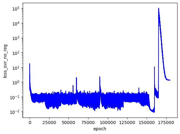
The "correctness" of each PINN is defined by the loss without $L_{trivial}$ ("loss_ovr_no_reg" in the plot below)
$$\begin{eqnarray} L = L_f + L_{bc} .\end{eqnarray}$$
I trained this PINN to search over the first three analytical $E$ values. I searched across three values for each $E$ and saved the three best PINNs.

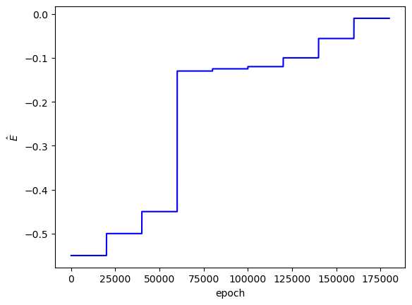
As I'd hoped, the best PINN convergence occurred when the correct analytical $E$ values were used as inputs: $E_1=-0.5$, $E_2=-0.125$, $E_3=-0.056$. Although the best PINNs used the correct $E$ values, the differences between $L$ across the adjacent $E$ values is not very significant (only an order of magnitude for each PINN).
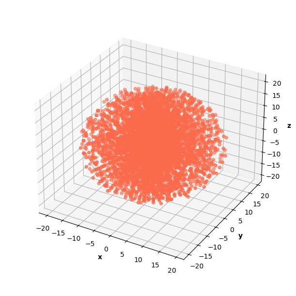
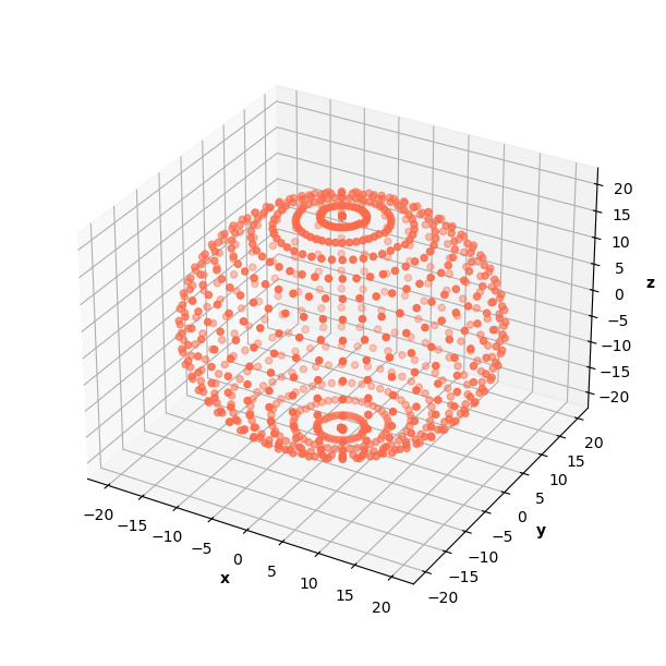
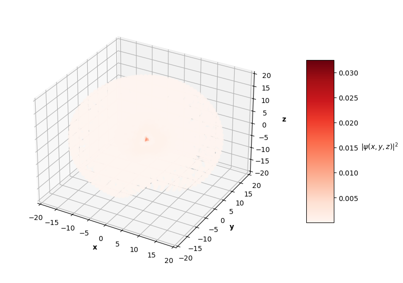
To visualize the solutions, I plot the square of the wavefunction's magnitude (effectively the probability density), $|\hat{\psi}(x, y, z)|^2$, for each $x$, $y$, $z$ in the sphere of data. I also cut a slice of the sphere away so you can see the distribution of predictions. The PINN can only converge to one of potentially many degenerate solutions for each energy level, so I pair the predictions up with the corresponding $nlm$ degenerate analytical solution below.
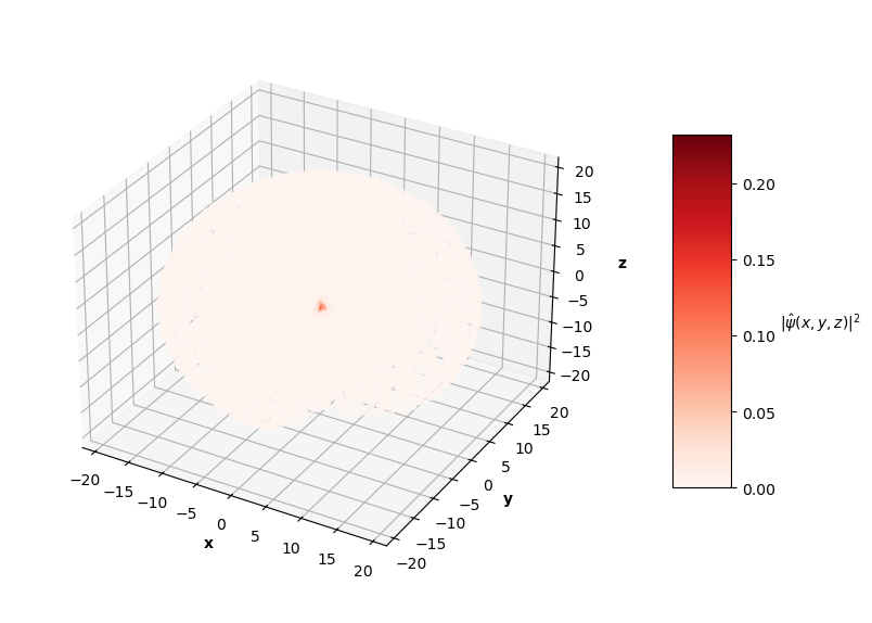
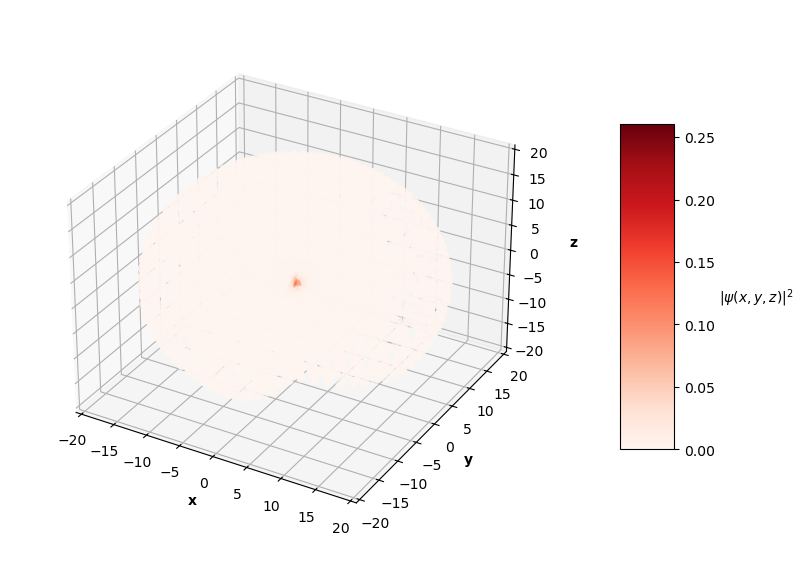

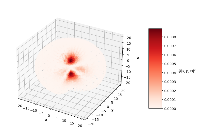
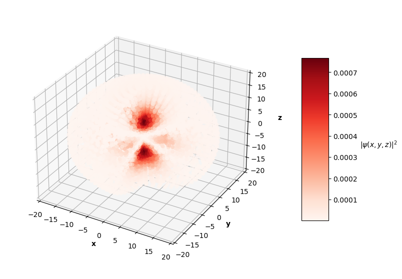
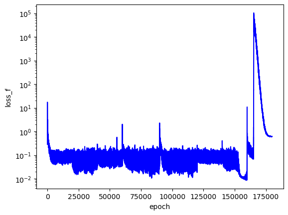
Qualitatively, the PINN was able to find solutions whose distribution of probability densities look similar to that of their corresponding analytical solutions. The best models attained $L$ values on the order of $10^{-2}$. Interestingly, the ground state model learned the boundary conditions the best with an $L_{bc}$ on the order of $10^{-5}$, while the $n=2$ and $n=3$ PINNs reached an order of $10^{-4}$. All PINNs attained an $L_f$ on the order of $10^{-2}$, which dominated their resulting total $L$. It looks as though these PINNs were able to find the correct solution at the boundary conditions with relative ease, but were not able to fit the rest of the wavefunction as accurately. Intuitively, this makes sense because the wavefunction at the boundary conditions is always 0, an easy mapping for the neural network to memorize.
This approach has its limitations. For each successive (higher energy) solution to the Hydrogen atom Schrodinger equation, the probability of the particle existing farther away from the nucleus increases, meaning a greater radius is needed to see the entire non-trivial part of the wavefunction. This presents a challenge in data generation. I generated a sphere of data with a maximum radius of 20. For the $n=1$ solution, points outside of the radius ~6 are mostly trivial and do not display any "meaningful" behavior for the PINN to learn. On the other hand, the $n=3$ wavefunction has non-trivial features up to a radius of ~15. I could have generated different size spheres for each PINN energy level to combat this issue, but I instead stuck to a single set of data with a fixed sphere size.
For the PINN approach to be useful for solving hard differential equations, it must be able to solve the problem given a limited number of constraints. Knowing that a larger sphere of data is needed to described the higher energy solutions requires knowledge about the analytical solution. For unsolved problems, this knowledge might not be available and assumptions would have to be made about the system modeled by the PINN. The assumptions required with my $E$ scan algorithm are the biggest weakness to this PINN approach. Ideally, the PINN could find $E$ and the wavefunction on its own, and the $E$ scan wouldn't be needed. Of course, the PINN's ability to learn is still limited by the assumptions formed when generating data for training. And once again, the $E$ scan algorithm is also limited by the amount of time you'd like to spend searching over $E$ values. Training PINNs on a wide, fine-grain range of $E$ values takes considerable time and cost (if you don't have a cool GPU cluster and a lot of money, that is. OpenAI could probably scan thousands of $E$ values in a few minutes).
Furthermore, I didn't spend much time trying to optimize the neural network's architecture or its hyperparameters. Better results could be obtained with these considerations. Additionally, the PINN could include constraints that consider other physical properties such as symmetry, conservation laws, and orthonormality between wavefunctions to achieve better convergence.
My code implementation for this problem can be found in this repo.
Next steps
I've claimed that this approach has limitations with scaling into harder problems that require actual assumptions. To test the effectiveness of this PINN approach, I'm now going to apply it to the Helium atom Schrodinger equation. This equation does not have an analytical solution and its wavefunction can only be approximated. It's not going to be easy and I don't know if I'll be able to get a PINN to learn anything meaningful, but I'm going to try nonetheless. See you in several weeks.